Function Transformations

Section 1.2 Function Transformations

In this section, we continue to look at ways to build new functions from existing ones. In the case of transformations, we will also examine how the graph of the new function relates to the original.

🔗

Goals:

🔗

F: Be able to determine a composition of functions given in any form (graph, table, equation).
🔗

🔗
F: Be able to perform arithmetic (sum, difference, product, quotient) on functions given in any form (graph, table, equation).
🔗

🔗
F: Be able to determine or describe a transformation (reflection, translation, dilation) of a function given in any form (graph, table, equation).
🔗

🔗

🔗

Problem 1.2.1.

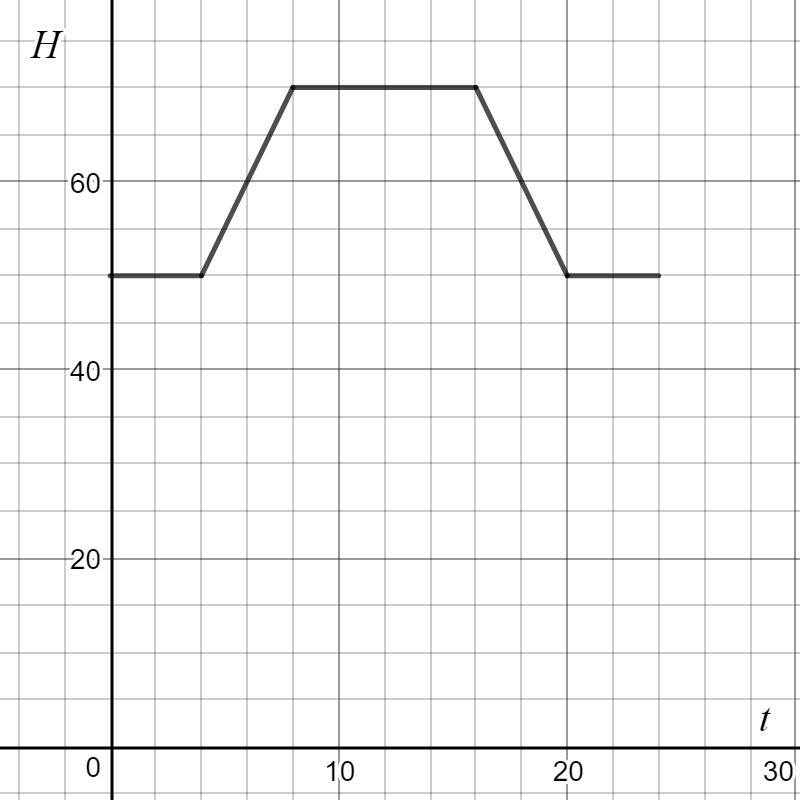
To save money, an office building is kept warm only during business hours. The graph below shows the temperature, $H$ in $^\circ F$ as a function of time $t\text{,}$ in hours after midnight. Suppose that the building’s superintendent decides to keep the building 5 $^\circ F$ warmer than before.

Adapted from Anton, H. (2003). Functions modeling change: A preparation for calculus, 2nd ed. John Wiley.

🔗

The graph of $H$ is a piecewise linear function over the interval $0 \le t \le 24\text{.}$ It starts at $H = 50\text{,}$ rises to $H = 70$ between $t = 4$ and $t = 8\text{,}$ remains constant at $H = 70$ until $t = 16\text{,}$ then decreases back to $H = 50$ by $t = 20\text{,}$ and stays at $H = 50$ for the remainder of the interval. The graph consists of horizontal and slanted segments forming a trapezoidal shape. — Figure 1.2.2. Graph of $H$ as a function of $t\text{.}$
🔗

🔗

On the graph above, sketch the graph $H_w$ ($H$ warmer) that shows the new temperature $t$ hours after midnight.
🔗

🔗
Write an equation for $H_w$ in terms of $H\text{.}$
🔗

🔗

🔗

Problem 1.2.3.

Suppose the same office building decides to start heating the building two hours earlier.

🔗

On the graph above, sketch the graph $H_e$ ($H$ earlier) that shows the new temperature $t$ hours after midnight.
🔗

🔗
Write an equation for $H_e$ in terms of $H\text{.}$
🔗

🔗

🔗

Problem 1.2.5.

The graph of $H(t)$ is a decreasing, concave-up curve resembling exponential decay. It begins at $(0, 100)\text{,}$ falls to $50$ by $t = 5\text{,}$ continues decreasing past $25$ at $t = 10\text{,}$ and approaches values close to $10$ by $t \approx 16\text{.}$ The rate of decrease slows over time. — Figure 1.2.6. Graph of $H(t)\text{.}$
🔗

In the human body, caffeine has a half life of approximately 5 hours. Figure 1.2.6 shows how much caffeine, $C$ (in mg) is left in Jeff’s bloodstream $t$ hours after 12 pm when he drinks a cup of coffee that contains 100 mg of caffeine. At 1 pm, his friend Carlos joins him and drinks a cup of coffee containing 100 mg of caffeine.

🔗

On Figure 1.2.6, sketch the graph of $C_l$ ($C$ later) that shows how much caffeine is in Carlos’ bloodstream $t$ hours after 12 pm.
🔗

🔗
Write an equation for $C_l$ in terms of $C\text{.}$
🔗

🔗

🔗

Problem 1.2.7.

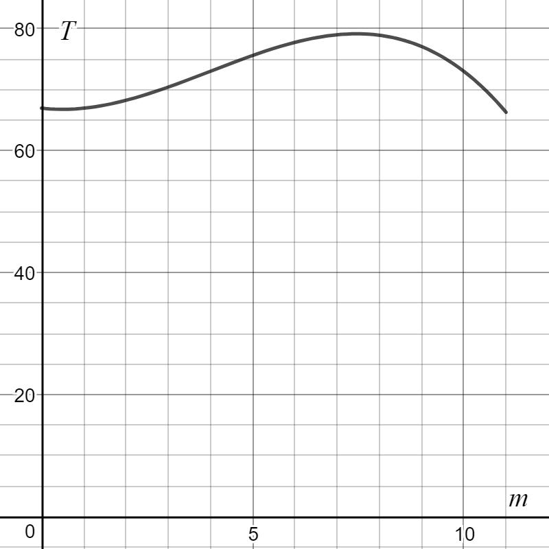
The graph in Figure 1.2.8 below shows the average daily high temperature, $T$ (in $F$), $m$ months after January in Carson, CA. San Francisco, CA is approximately 5 degrees cooler than Carson.

🔗

The graph of $T$ is a smooth curve that starts near $T = 66$ at $m = 0\text{,}$ rises gradually, and reaches a maximum of about $T = 80$ near $m \approx 7\text{.}$ After the peak, the curve decreases slightly, ending near $T = 66$ at $m = 11\text{.}$ The overall shape is a gentle rise and fall, indicating a single peak. — Figure 1.2.8. Graph of $T$ as a function of $m\text{.}$
🔗

On the graph above, sketch the graph of $T_c$ ($T$ cooler) that shows the average high temperature $m$ months after January in San Francisco.
🔗

🔗
Write an equation for $T_c$ in terms of $T\text{.}$
🔗

🔗

🔗

Problem 1.2.9.

Write a rule that generalizes your observations about vertical shifts from the above problems.

🔗

Problem 1.2.10.

Write a rule that generalizes your observations about horizontal shifts from the above problems.

🔗

Problem 1.2.11.

For each problem below (i) Write a function equation for the indicated function in terms of $f(x)\text{,}$ (ii) Write a function equation for for the indicated function in terms of $x\text{,}$ (iii) Use your knowledge of basic functions and translations to sketch the graph, (iv) Check your graph using Desmos.

🔗

Let $f(x)=\sqrt{x}\text{.}$ $g(x)$ is a function whose graph is the graph of $f(x)$ shifted left 3 units.
$A blank Cartesian coordinate grid with bold horizontal and vertical axes intersecting at the origin. The horizontal axis is labeled from $-10$ to $10\text{,}$ and the vertical axis is labeled from $-5$ to $10\text{.}$ The grid consists of evenly spaced squares, ready for plotting points or graphs.$

Figure 1.2.12. Blank coordinate grid.
🔗
🔗

🔗
Let $f(x)=x^2\text{.}$ $k(x)$ is a function whose graph is the graph of $f(x)$ shifted down 2 units and right 4 units.
$A blank Cartesian coordinate grid with bold horizontal and vertical axes intersecting at the origin. The horizontal axis is labeled from $-10$ to $10\text{,}$ and the vertical axis is labeled from $-5$ to $10\text{.}$ The grid consists of evenly spaced squares, ready for plotting points or graphs.$

Figure 1.2.13. Blank coordinate grid.
🔗
🔗

🔗

🔗

Problem 1.2.14.

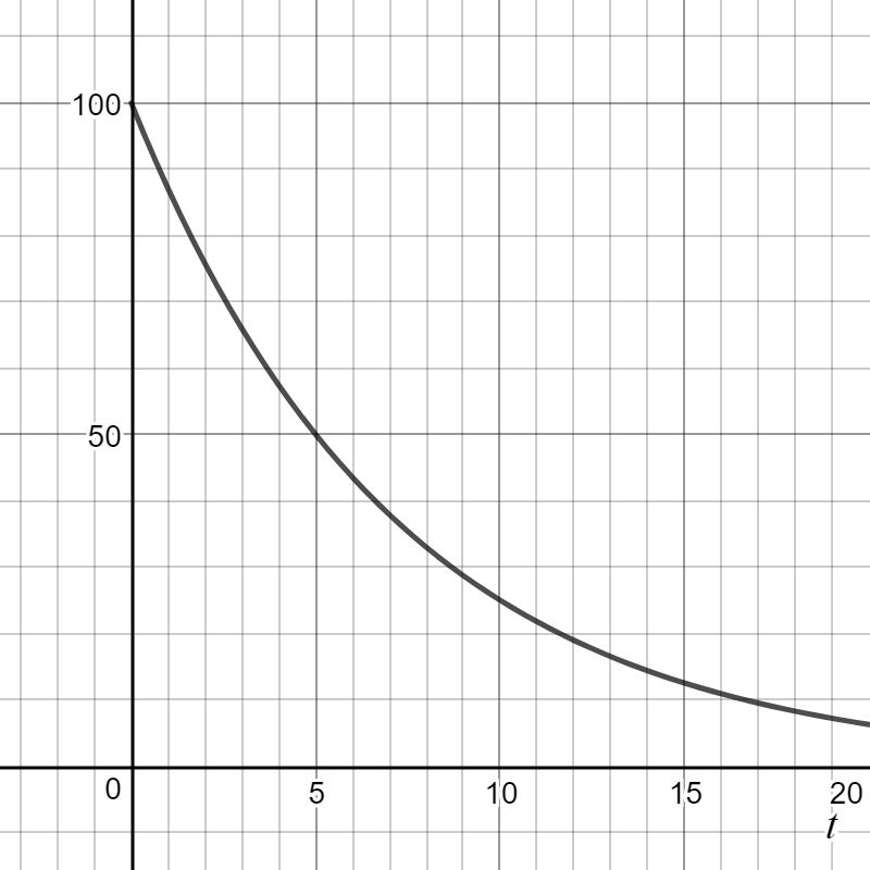
In the human body, caffeine has a half life of approximately 5 hours. The graph below shows how much caffeine, $C$ (in mg) is left in Jeff’s bloodstream $t$ hours after 12 pm when he drinks a cup of coffee that contains 100 mg of caffeine. Jeff’s friend Monica has a half-caff (a cup of coffee with half the amount of caffeine, 50 mg).

🔗

A curve starting at 100 on the vertical axis, passing through $(5,50)$ and decreasing toward zero as time $t$ increases from 0 to 20. The horizontal axis is labeled $t\text{,}$ and the vertical axis shows values from 0 to 100. — Figure 1.2.15. Graph of an exponential decay function over time.
🔗

On the graph above, sketch the graph of $C_h$ ($C$ half) that shows how much caffeine is in Monica’s bloodstream $t$ hours after 12 pm.
🔗

🔗
Write an equation for $C_h$ in terms of $C\text{.}$
🔗

🔗

🔗

Problem 1.2.16.

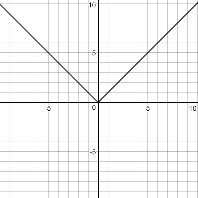
$y(x)=|x|$ is graphed below.

🔗

A V-shaped graph representing the function $y = |x|\text{.}$ The vertex is at the origin (0, 0), with one ray extending upward to the right through (10, 10) and the other upward to the left through (-10, 10). The axes are labeled with values from -10 to 10. — Figure 1.2.17. Graph of the absolute value function.
🔗

Building on what you have learned so far, add the graph of $z(x)=-y(x)$ to the graph of above. Check your graph using Desmos.
🔗

🔗
Write a function equation in terms of $x$ for $z(x)\text{.}$
🔗

🔗

🔗

Problem 1.2.18.

Let $g(x)=af(x)\text{.}$ Based on what you learned from Problem 1.2.14 and Problem 1.2.16, explain the role of $a$ in transforming $f(x)$ into $g(x)\text{.}$

🔗

Problem 1.2.19.

For each problem below (i) Describe the transformations required (in the correct order) to transform the first function into the second, (ii) Write a function equation for for the indicated function in terms of $x\text{,}$ (iii) Use your knowledge of basic functions and translations to sketch the graph, (iv) Check your graph using Desmos.

🔗

$m(x)=2^{x}\text{,}$ $k(x)=-m(x)-3$

Figure 1.2.20. Blank coordinate plane with grid lines.
🔗
🔗

🔗
Let $n(x)=x^3\text{,}$ $t(x)=2n(x-1)+2$

Figure 1.2.21. Blank coordinate plane with grid lines.
🔗
🔗

🔗

🔗

Prev Top Next