Section 2.3 Comparing Linear and Exponential Models

Both linear and exponential functions are often used to model real data. In this section, we will explore how each of these models works in the context of population data.
Goals:
  • E: Be able to model a situation with appropriate exponential equation(s) and interpret the solution.
  • E: Be able to determine the equation of an exponential function given a table of values.
  • F: Be able to determine an appropriate function class (linear, quadratic, exponential, trigonometric) to model a particular situation.
  • F: Be able to compute the average rate of change of a given function on a given interval

Definition 2.3.1.

The average rate of change of a function \(h\) defined on an interval \(a \leq x \leq b\) is
\begin{equation*} \frac{h(b)-h(a)}{b-a}. \end{equation*}
Note that the average rate of change computes the slope of the line between the two points \((a,h(a))\) and \((b,h(b))\text{.}\)

Investigation 2.3.1.

In Exercise Set 1, FigureΒ 1.1.13, we saw that the height above the ground, \(h\) of a ball \(t\) seconds after being dropped off a 60 meter tall building is given by the equation \(h(t)=-4.9t^2+60\) and is shown on the graph below.
  1. Between when the ball is dropped and when it hits the ground, does it fall at a constant rate? Why or why not?
  2. How far does the ball fall between \(t=0\) and \(t=3\) seconds?
  3. What is the average rate of change of the ball between \(t=0\) and \(t=3\) seconds? Write an algebraic expression using function notation for the average rate of change, then compute it.
  4. What are the units of the change in height of the ball? What are the units in the change in time? What are the units for the average rate of change you computed in ItemΒ 3?
  5. What is the average rate of change of the ball between the time it is dropped off the building and the time it hits the ground? Be sure to include units in your answer.

Definition 2.3.2.

A function \(h\) is increasing on the interval \(a \leq x \leq b\) if, whenever two points \(c\) and \(d\) are in the interval, with \(c<d\text{,}\) then \(f(c)<f(d)\text{.}\) A function \(h\) is decreasing on the interval \(a \leq x \leq b\) if, whenever two points \(c\) and \(d\) are in the interval, with \(c<d\text{,}\) then \(f(c)>f(d)\text{.}\)
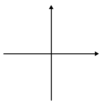
Informally, the definitions for increasing and decreasing are stating that if a function goes up as we move from left to right, it is increasing, and if it goes down as we move from left to right, it is decreasing.Below, sketch a function that is increasing on \((- \infty, \infty)\) and a function that is decreasing on \((- \infty, \infty)\text{.}\)
Blank coordinate grid for sketching an increasing function.
Blank coordinate grid for sketching a decreasing function.
Figure 2.3.3. Sketches of an increasing function and a decreasing function.

Example 2.3.4.

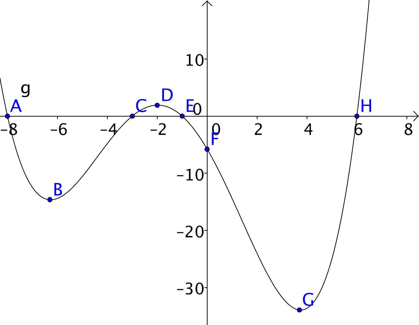
Refer to the graph and table for \(g\) in FigureΒ 2.3.5.
Graph of the function g with labeled points A through H.
Label \(A\) \(B\) \(C\) \(D\) \(E\) \(F\) \(G\) \(H\)
\(x\) \(-8\) \(-6.3\) \(-3\) \(-2\) \(-1\) \(0\) \(3.7\) \(6\)
\(g(x)\) \(0\) \(-14.6\) \(0\) \(1.9\) \(0\) \(-5.8\) \(-33.9\) \(0\)
(a) Table for \(g\)
Figure 2.3.5. Graph and table for \(g\text{.}\)
  1. Find the average rate of change of \(g\) on the interval \(-6.3 \leq x \leq 3.7\text{.}\)
  2. Find the average rate of change of \(f\) on the interval \(-8 \leq x \leq 6\text{.}\)
  3. On what intervals is \(g\) increasing? On what intervals is \(g\) decreasing?
Solution.
The solution to ExampleΒ 2.3.4 is outlined below:
The function we are given goes down (is decreasing) from point \(A\) to point \(B\text{,}\) then increases from point \(B\) to point \(D\text{,}\) decreases again from point \(D\) to point \(G\text{,}\) and then increases from point \(G\) to point \(H\) and beyond.
In this case, we only have the graph, and not the equation, so we should not make assumptions about what happens outside of the interval \(-8 \leq x \leq 6\text{.}\) Thus, \(g\) is increasing on the intervals \(-6.3 \leq x \leq -2\text{,}\) and again on \(3.7 \leq x \leq 6\text{.}\) The function \(g\) is decreasing on the intervals \(-8 \leq x \leq -6.3\) and \(-2 \leq x \leq 3.7\text{.}\)
The average rate of change of \(g\) on the interval \(-6.3 \leq x \leq 3.7\) is \(\frac{-33.9-(-14.6)}{3.7-(-6.3)}=\frac{-19.3}{10}=1.93\text{.}\) The average rate of change of \(g\) on the interval \(-8 \leq x \leq 6\) is \(\frac{0-0}{6-(-8)}=0\text{.}\)
Can you explain why the average rate of change was 0 on the interval \(-8 \leq x \leq 6\text{?}\)
Problem 2.3.6.

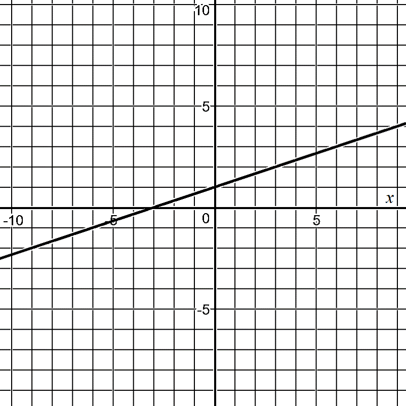
  1. Using the graph of \(f(x)=\frac{1}{3}x+1\) below, choose two points on the graph and find the average rate of change between those two points.
    A coordinate grid showing a straight line with positive slope. The line rises from left to right, crossing the y-axis at y equals 1 and crossing the x-axis at x equals negative 3.
    Figure 2.3.7. Graph of the linear function \(f(x)=\frac{1}{3}x+1\text{.}\)
  2. Choose two different points on the graph of \(f(x)=\frac{1}{3}x+1\) above and find the average rate of change between those two points.
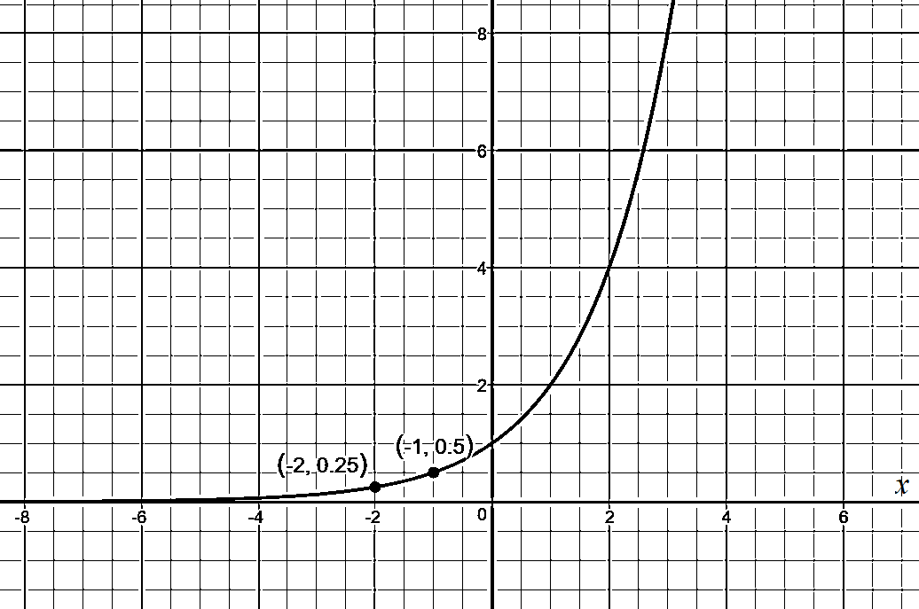
  3. Using the graph of \(g(x)=2^x\) below, choose two points on the graph and find the average rate of change between those two points.
    A coordinate grid showing an exponential curve that increases slowly for negative x-values and then rises rapidly for positive x-values. The curve passes through the points (-2, 0.25), (-1, 0.5), and (0, 1), illustrating exponential growth.
    Figure 2.3.8. Graph of the exponential function \(g(x)=2^x\text{.}\)
  4. Choose two different points on the graph of \(g(x)=2^x\) above and find the average rate of change between those two points.
  5. Summarize what you have learned about how linear functions like \(f\) from ItemΒ 1 and exponential functions like \(g\) from ItemΒ 3 are different in terms of their rates of change.

Investigation 2.3.2.

You have been hired as a consultant for the City of Los Angeles. City planners need to understand population data and use the data to predict the population in the future. Having a good estimate of the city’s population helps the planners decide how much money will be needed for city maintenance and services, and helps local officials anticipate the needs for housing, school and other construction, and much more. Your work begins with finding the population of Los Angeles in the United States Census for 1920 to 2010. This data appears in TableΒ 2.3.9.
Table 2.3.9. U.S. Census Bureau data for Los Angeles (city), 1920-2010
\(x\) (yrs since 1920) Year Actual Pop. Pop. Using Linear Model Pop. Using Exponential Model
0 1920 576,673
10 1930 1,238,048
20 1940 1,504,277
30 1950 1,970,358
40 1960 2,479,015
50 1970 2,816,061
60 1980 2,966,850
70 1990 3,485,398
80 2000 3,694,820
90 2010 3,792, 621
  1. Linear Model. One way to model a population is with a linear function, \(y=mx+b\text{,}\) where \(m\) and \(b\) are real numbers. As a first attempt, find the equation of the line passing through the data for 1920 and 2010.
  2. Use your linear model from ItemΒ 1 to put the estimated population for values \(t=0\) to \(t=90\) into TableΒ 2.3.9 . How do the values compare with the actual data?
  3. At this url: https://goo.gl/dynoa2, you will find Desmos set up with the data. Using Desmos, find the values of \(m\) and \(b\) that you think make the line \(y=mx+b\) best fit the data. Make a note of the equation. How does the equation compare to your linear model from ItemΒ 1? How does the equation look compared to the actual data points on the graph?
  4. Exponential Model. Find the equation of an exponential model passing through the data for 1920 \((t=0)\) and 2010 \((t=90)\text{.}\)
  5. Use your exponential model from ItemΒ 4 to add the estimated population for values \(t=0\) to \(t=90\) to TableΒ 2.3.9 . How do the values compare with the actual data?
  6. Graph the exponential model \(G(x)=945802(1.01845)^x\) in Desmos. How does the equation compare to your own linear model from ItemΒ 1? How does the best-fit equation look compared to the actual data points on the graph?
  7. Comparing the models. Your final job is to make a decision about which model will best predict the population over the next ten to twenty years. Justify your decision based on both mathematics and what you know or think will happen in Los Angeles.

Problem 2.3.10.

For each table or situation below, identify which class of function (linear, quadratic or exponential) you would choose to model that table or situation, and explain why. Then write a function equation for each table or situation.
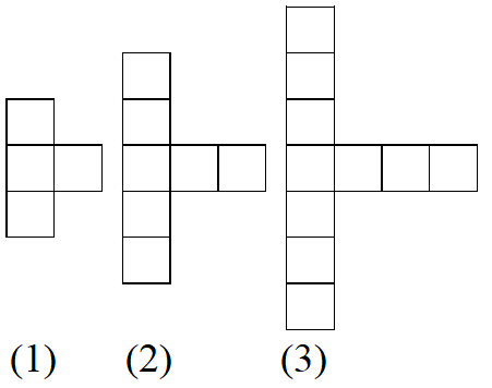
  1. Let \(t(n)\) be a function that gives the number of squares in the nth figure for the pattern shown below.
    Three growing square patterns labeled (1), (2), and (3). Each figure consists of a vertical column of squares with a horizontal arm extending to the right. The number of squares increases from Figure (1) to Figure (3).
    Figure 2.3.11. Square patterns for Figures (1), (2), and (3).
  2. Table 2.3.12.
    \(x\) \(-4\) \(-2\) 0 2 4
    \(g(x)\) 48 12 3 0.75 0.1875
  3. A breeder keeps pet rabbits. In January he has 20 rabbits. His population of rabbits doubles every 3 months. Let \(P\text{,}\) the population of rabbits, be a function of \(t\text{,}\) the number of months since January.
  4. Table 2.3.13.
    \(x\) \(-6\) \(-3\) 0 3 6
    \(f(x)\) 600 100 \(-400\) \(-900\) \(-1400\)
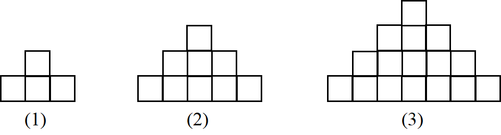
  5. Let \(k(n)\) be a function that gives the number of squares in the nth figure for the pattern shown below.
    Three stepped square patterns labeled (1), (2), and (3). Figure (1) has a base row of three squares with one square centered above. Figure (2) has a wider base with two stacked rows above it, and Figure (3) shows a larger stepped pyramid with three levels above the base. The number of squares increases from left to right.
    Figure 2.3.14. Square patterns for Figures (1), (2), and (3).
  6. Chris has $150 on his meal card. Every time he orders a meal, $9 is deducted from his card. Let \(M\text{,}\) the balance Chris has on his meal card, be a function of \(n\text{,}\) the number of meals he has ordered.